
🤔 PHASE 1: ASK
Introduction
This study analyses the differences in behaviour between casual riders and annual members of Cyclistic Bike-Share, using data science techniques to uncover usage patterns. The goal is to support Cyclistic’s strategy of increasing annual memberships, as they are more profitable. Insights from the analysis will guide a targeted marketing campaign to convert casual users into annual members, helping the company grow inclusively and sustainably.
Company Background
Cyclistic, based in Chicago, provides a bike-share program with a fleet of bicycles available for public use across the city. They offer single-ride, full-day, and annual memberships. Operating on a subscription-based model, Cyclistic caters to both casual riders and annual members, emphasising an inclusive and accessible transportation option for diverse user groups.
Business Task: The objective is to analyse Cyclistic’s historical bike trip data to identify differences in how casual riders and annual members use the service. The insights from this analysis will inform a new marketing strategy aimed at encouraging casual riders to transition into annual members.
Key Stakeholders
| Stakeholder | Role |
|---|---|
| Lily Moreno | The director of marketing and your manager. Responsible for developing campaigns. |
| Cyclistic Marketing Analytics Team | Tasked with gathering, analysing, and reporting data to support marketing strategies. |
| Cyclistic Executive Team | Responsible for reviewing and approving the proposed marketing initiatives. |
Key Questions
- What are the differences in bike usage patterns between casual riders and annual members?
- Which unique behaviours of casual riders can be addressed through targeted marketing efforts?
- What trends or seasonal patterns exist between the two user groups, and how can these influence the timing of marketing campaigns?
Assumptions and Limitations
Assumptions:
- The dataset is accurate, up-to-date, and representative of the broader rider population.
- User behaviours are primarily influenced by their rider type (casual vs. annual members) and not by unrecorded factors.
Limitations:
- The dataset provides extensive ride details but lacks demographic information such as age, gender, and socioeconomic status.
- Analysis and conclusions rely solely on ride patterns, without accounting for potential demographic influences.

👩🍳 PREPARE PHASE
Data Location and Organisation
- Data Source: Motivate International Inc.
- Availability: Publicly available for download.
- Format: CSV.
- Structure: Each row represents a bike trip, and columns contain information such as:
- Trip duration
- Start time
- End time
- Departure station
- Arrival station
- Bike type
- User type (casual or member)
- Action Taken: The provided code downloads and combines data from multiple CSV files into a single DataFrame called
merged_df.
Data Credibility and Bias
- Credibility: Considered high, as the data is provided by the company operating the service.
- Bias: Recognition of potential biases due to operational constraints or data collection methods. For example, the data represents only users of the Cyclistic service and may not be representative of all cyclists in Chicago.
Licensing, Privacy, Security, and Accessibility
- Licensing: The data is provided under a specific license that allows analysis but prohibits sharing as a stand-alone dataset.
- Privacy: Preserved as there is no personally identifiable information in the data.
- Security: Involves storing the downloaded data in a secure, potentially encrypted location.
- Accessibility: Ensuring that the data and subsequent analysis are available to all project stakeholders.
Data Integrity
- Verification: The data will be verified for integrity using Exploratory Data Analysis (EDA) to identify inconsistencies, missing values, outliers, or duplicate entries.
- Action Taken: The code identifies the number of missing values per column using the
missingnolibrary.
Relevance to the Business Question
The data contains information about trips by casual users and annual members, which is directly relevant to the business question of understanding how the two types of users use Cyclistic bikes differently. Analysing this data can provide insights to inform a marketing strategy aimed at converting casual users into annual members.
Potential Issues
Potential issues include:
- Missing data
- Errors in the data
- Bias
The data may not contain additional useful information, such as demographic details of users or specific reasons for choosing casual travel over a subscription.
Key Tasks
- Download the data and store it appropriately: The provided code accomplishes this task by downloading and storing the data in a DataFrame.
- Identify how the data is organised: Explore the dataset to understand its structure and what each column represents.
# Define the base URL
base_url <- "https://divvy-tripdata.s3.amazonaws.com/"

# Define the list of zip files to download
zip_files <- c(
  "Divvy_Trips_2020_Q1.zip",
  "Divvy_Trips_2019_Q4.zip",
  "Divvy_Trips_2019_Q3.zip",
  "Divvy_Trips_2019_Q2.zip"
)

# Create a directory to store the files
if (!dir.exists("divvy_data")) {
  dir.create("divvy_data")
}

# Loop through the zip files and download/unzip them
for (file in zip_files) {
  file_url <- paste0(base_url, file)
  dest_file <- file.path("divvy_data", file)  # Save to the 'divvy_data' directory

  # Download the file
  download.file(file_url, destfile = dest_file, mode = "wb")

  # Unzip the file
  unzip(dest_file, exdir = "divvy_data")  # Extract to the 'divvy_data' directory

  # Remove the zip file after unzipping (optional)
  file.remove(dest_file)
}

print("Files downloaded and unzipped successfully!")
[1] "Files downloaded and unzipped successfully!"# Downloading necessary packages
install.packages(c("tidyverse", "lubridate", "skimr", "janitor", "ggplot2"))
# Load the packages
library(tidyverse) # For data manipulation and visualization
library(lubridate) # For date-time handling
library(skimr) # For summary statistics
library(janitor) # For cleaning column names
library(ggplot2) # For plots
library(dplyr) # For data wranglingInstalling packages into ‘/usr/local/lib/R/site-library’
(as ‘lib’ is unspecified)
also installing the dependency ‘snakecase’
── [1mAttaching core tidyverse packages[22m ──────────────────────── tidyverse 2.0.0 ──
[32m✔[39m [34mdplyr [39m 1.1.4 [32m✔[39m [34mreadr [39m 2.1.5
[32m✔[39m [34mforcats [39m 1.0.0 [32m✔[39m [34mstringr [39m 1.5.1
[32m✔[39m [34mggplot2 [39m 3.5.2 [32m✔[39m [34mtibble [39m 3.2.1
[32m✔[39m [34mlubridate[39m 1.9.4 [32m✔[39m [34mtidyr [39m 1.3.1
[32m✔[39m [34mpurrr [39m 1.0.4
── [1mConflicts[22m ────────────────────────────────────────── tidyverse_conflicts() ──
[31m✖[39m [34mdplyr[39m::[32mfilter()[39m masks [34mstats[39m::filter()
[31m✖[39m [34mdplyr[39m::[32mlag()[39m masks [34mstats[39m::lag()
[36mℹ[39m Use the conflicted package ([3m[34m<http://conflicted.r-lib.org/>[39m[23m) to force all conflicts to become errors
Attaching package: ‘janitor’
The following objects are masked from ‘package:stats’:
chisq.test, fisher.test# Now that iI have downloaded the files and packages, I need to create paths for the datasets
files <- list.files(path = "/content/divvy_data", pattern = "*.csv", full.names = TRUE)
length(files)
print(files)4
[1] "/content/divvy_data/Divvy_Trips_2019_Q2.csv"
[2] "/content/divvy_data/Divvy_Trips_2019_Q3.csv"
[3] "/content/divvy_data/Divvy_Trips_2019_Q4.csv"
[4] "/content/divvy_data/Divvy_Trips_2020_Q1.csv"
# Here, I want to understand the column's names.
library(dplyr)
# File paths
files <- c(
"/content/divvy_data/Divvy_Trips_2019_Q2.csv",
"/content/divvy_data/Divvy_Trips_2019_Q3.csv",
"/content/divvy_data/Divvy_Trips_2019_Q4.csv",
"/content/divvy_data/Divvy_Trips_2020_Q1.csv"
)
# Function to get column names from a CSV file
get_column_names <- function(file_path) {
tryCatch({
readr::read_csv(file_path, n_max = 1) %>% names()
}, error = function(e) {
message(paste("Error reading file", file_path, ":", e$message))
return(NULL) # Return NULL if there is an error
})
}
# Get column names for each file
all_columns <- lapply(files, get_column_names)
# Print column names of each file
for (i in seq_along(files)){
cat("Columns for file: ", files[i], "\n")
print(all_columns[[i]])
cat("\n")
}[1mRows: [22m[34m1[39m [1mColumns: [22m[34m12[39m
[36m──[39m [1mColumn specification[22m [36m────────────────────────────────────────────────────────[39m
[1mDelimiter:[22m ","
[31mchr[39m (4): 03 - Rental Start Station Name, 02 - Rental End Station Name, User...
[32mdbl[39m (6): 01 - Rental Details Rental ID, 01 - Rental Details Bike ID, 01 - R...
[34mdttm[39m (2): 01 - Rental Details Local Start Time, 01 - Rental Details Local En...
[36mℹ[39m Use `spec()` to retrieve the full column specification for this data.
[36mℹ[39m Specify the column types or set `show_col_types = FALSE` to quiet this message.
[1mRows: [22m[34m1[39m [1mColumns: [22m[34m12[39m
[36m──[39m [1mColumn specification[22m [36m────────────────────────────────────────────────────────[39m
[1mDelimiter:[22m ","
[31mchr[39m (4): from_station_name, to_station_name, usertype, gender
[32mdbl[39m (5): trip_id, bikeid, from_station_id, to_station_id, birthyear
[32mnum[39m (1): tripduration
[34mdttm[39m (2): start_time, end_time
[36mℹ[39m Use `spec()` to retrieve the full column specification for this data.
[36mℹ[39m Specify the column types or set `show_col_types = FALSE` to quiet this message.
[1mRows: [22m[34m1[39m [1mColumns: [22m[34m12[39m
[36m──[39m [1mColumn specification[22m [36m────────────────────────────────────────────────────────[39m
[1mDelimiter:[22m ","
[31mchr[39m (4): from_station_name, to_station_name, usertype, gender
[32mdbl[39m (6): trip_id, bikeid, tripduration, from_station_id, to_station_id, bir...
[34mdttm[39m (2): start_time, end_time
[36mℹ[39m Use `spec()` to retrieve the full column specification for this data.
[36mℹ[39m Specify the column types or set `show_col_types = FALSE` to quiet this message.
[1mRows: [22m[34m1[39m [1mColumns: [22m[34m13[39m
[36m──[39m [1mColumn specification[22m [36m────────────────────────────────────────────────────────[39m
[1mDelimiter:[22m ","
[31mchr[39m (5): ride_id, rideable_type, start_station_name, end_station_name, memb...
[32mdbl[39m (6): start_station_id, end_station_id, start_lat, start_lng, end_lat, e...
[34mdttm[39m (2): started_at, ended_at
[36mℹ[39m Use `spec()` to retrieve the full column specification for this data.
[36mℹ[39m Specify the column types or set `show_col_types = FALSE` to quiet this message.
Columns for file: /content/divvy_data/Divvy_Trips_2019_Q2.csv
[1] "01 - Rental Details Rental ID"
[2] "01 - Rental Details Local Start Time"
[3] "01 - Rental Details Local End Time"
[4] "01 - Rental Details Bike ID"
[5] "01 - Rental Details Duration In Seconds Uncapped"
[6] "03 - Rental Start Station ID"
[7] "03 - Rental Start Station Name"
[8] "02 - Rental End Station ID"
[9] "02 - Rental End Station Name"
[10] "User Type"
[11] "Member Gender"
[12] "05 - Member Details Member Birthday Year"
Columns for file: /content/divvy_data/Divvy_Trips_2019_Q3.csv
[1] "trip_id" "start_time" "end_time"
[4] "bikeid" "tripduration" "from_station_id"
[7] "from_station_name" "to_station_id" "to_station_name"
[10] "usertype" "gender" "birthyear"
Columns for file: /content/divvy_data/Divvy_Trips_2019_Q4.csv
[1] "trip_id" "start_time" "end_time"
[4] "bikeid" "tripduration" "from_station_id"
[7] "from_station_name" "to_station_id" "to_station_name"
[10] "usertype" "gender" "birthyear"
Columns for file: /content/divvy_data/Divvy_Trips_2020_Q1.csv
[1] "ride_id" "rideable_type" "started_at"
[4] "ended_at" "start_station_name" "start_station_id"
[7] "end_station_name" "end_station_id" "start_lat"
[10] "start_lng" "end_lat" "end_lng"
[13] "member_casual"# Here I want to understand its structure and what each column represents
# Function to read and glimpse a CSV file
glimpse_file <- function(file_path) {
tryCatch({
df <- readr::read_csv(file_path)
glimpse(df)
return(df) # Return the dataframe if needed later
}, error = function(e) {
message(paste("Error reading file", file_path, ":", e$message))
return(NULL) # Return NULL in case of error
})
}
# Loop through the files and get a glimpse
for (file in files) {
cat("Structure for file:", file, "\n")
glimpse_file(file)
cat("\n")
}Structure for file: /content/divvy_data/Divvy_Trips_2019_Q2.csv
[1mRows: [22m[34m1108163[39m [1mColumns: [22m[34m12[39m
[36m──[39m [1mColumn specification[22m [36m────────────────────────────────────────────────────────[39m
[1mDelimiter:[22m ","
[31mchr[39m (4): 03 - Rental Start Station Name, 02 - Rental End Station Name, User...
[32mdbl[39m (5): 01 - Rental Details Rental ID, 01 - Rental Details Bike ID, 03 - R...
[32mnum[39m (1): 01 - Rental Details Duration In Seconds Uncapped
[34mdttm[39m (2): 01 - Rental Details Local Start Time, 01 - Rental Details Local En...
[36mℹ[39m Use `spec()` to retrieve the full column specification for this data.
[36mℹ[39m Specify the column types or set `show_col_types = FALSE` to quiet this message.
Rows: 1,108,163
Columns: 12
$ `01 - Rental Details Rental ID` [3m[90m<dbl>[39m[23m 22178529[90m, [39m22178530[90m,[39m…
$ `01 - Rental Details Local Start Time` [3m[90m<dttm>[39m[23m 2019-04-01 00:02:2…
$ `01 - Rental Details Local End Time` [3m[90m<dttm>[39m[23m 2019-04-01 00:09:4…
$ `01 - Rental Details Bike ID` [3m[90m<dbl>[39m[23m 6251[90m, [39m6226[90m, [39m5649[90m, [39m4…
$ `01 - Rental Details Duration In Seconds Uncapped` [3m[90m<dbl>[39m[23m 446[90m, [39m1048[90m, [39m252[90m, [39m357…
$ `03 - Rental Start Station ID` [3m[90m<dbl>[39m[23m 81[90m, [39m317[90m, [39m283[90m, [39m26[90m, [39m2…
$ `03 - Rental Start Station Name` [3m[90m<chr>[39m[23m "Daley Center Plaza…
$ `02 - Rental End Station ID` [3m[90m<dbl>[39m[23m 56[90m, [39m59[90m, [39m174[90m, [39m133[90m, [39m1…
$ `02 - Rental End Station Name` [3m[90m<chr>[39m[23m "Desplaines St & Ki…
$ `User Type` [3m[90m<chr>[39m[23m "Subscriber"[90m, [39m"Subs…
$ `Member Gender` [3m[90m<chr>[39m[23m "Male"[90m, [39m"Female"[90m, [39m"…
$ `05 - Member Details Member Birthday Year` [3m[90m<dbl>[39m[23m 1975[90m, [39m1984[90m, [39m1990[90m, [39m1…
Structure for file: /content/divvy_data/Divvy_Trips_2019_Q3.csv
[1mRows: [22m[34m1640718[39m [1mColumns: [22m[34m12[39m
[36m──[39m [1mColumn specification[22m [36m────────────────────────────────────────────────────────[39m
[1mDelimiter:[22m ","
[31mchr[39m (4): from_station_name, to_station_name, usertype, gender
[32mdbl[39m (5): trip_id, bikeid, from_station_id, to_station_id, birthyear
[32mnum[39m (1): tripduration
[34mdttm[39m (2): start_time, end_time
[36mℹ[39m Use `spec()` to retrieve the full column specification for this data.
[36mℹ[39m Specify the column types or set `show_col_types = FALSE` to quiet this message.
Rows: 1,640,718
Columns: 12
$ trip_id [3m[90m<dbl>[39m[23m 23479388[90m, [39m23479389[90m, [39m23479390[90m, [39m23479391[90m, [39m23479392[90m, [39m23…
$ start_time [3m[90m<dttm>[39m[23m 2019-07-01 00:00:27[90m, [39m2019-07-01 00:01:16[90m, [39m2019-07-0…
$ end_time [3m[90m<dttm>[39m[23m 2019-07-01 00:20:41[90m, [39m2019-07-01 00:18:44[90m, [39m2019-07-0…
$ bikeid [3m[90m<dbl>[39m[23m 3591[90m, [39m5353[90m, [39m6180[90m, [39m5540[90m, [39m6014[90m, [39m4941[90m, [39m3770[90m, [39m5442[90m, [39m2957…
$ tripduration [3m[90m<dbl>[39m[23m 1214[90m, [39m1048[90m, [39m1554[90m, [39m1503[90m, [39m1213[90m, [39m310[90m, [39m1248[90m, [39m1550[90m, [39m1583[90m,[39m…
$ from_station_id [3m[90m<dbl>[39m[23m 117[90m, [39m381[90m, [39m313[90m, [39m313[90m, [39m168[90m, [39m300[90m, [39m168[90m, [39m313[90m, [39m43[90m, [39m43[90m, [39m511[90m,[39m…
$ from_station_name [3m[90m<chr>[39m[23m "Wilton Ave & Belmont Ave"[90m, [39m"Western Ave & Monroe St…
$ to_station_id [3m[90m<dbl>[39m[23m 497[90m, [39m203[90m, [39m144[90m, [39m144[90m, [39m62[90m, [39m232[90m, [39m62[90m, [39m144[90m, [39m195[90m, [39m195[90m, [39m84[90m, [39m…
$ to_station_name [3m[90m<chr>[39m[23m "Kimball Ave & Belmont Ave"[90m, [39m"Western Ave & 21st St"…
$ usertype [3m[90m<chr>[39m[23m "Subscriber"[90m, [39m"Customer"[90m, [39m"Customer"[90m, [39m"Customer"[90m, [39m"C…
$ gender [3m[90m<chr>[39m[23m "Male"[90m, [39m[31mNA[39m[90m, [39m[31mNA[39m[90m, [39m[31mNA[39m[90m, [39m[31mNA[39m[90m, [39m"Male"[90m, [39m[31mNA[39m[90m, [39m[31mNA[39m[90m, [39m[31mNA[39m[90m, [39m[31mNA[39m[90m, [39m[31mNA[39m[90m, [39m…
$ birthyear [3m[90m<dbl>[39m[23m 1992[90m, [39m[31mNA[39m[90m, [39m[31mNA[39m[90m, [39m[31mNA[39m[90m, [39m[31mNA[39m[90m, [39m1990[90m, [39m[31mNA[39m[90m, [39m[31mNA[39m[90m, [39m[31mNA[39m[90m, [39m[31mNA[39m[90m, [39m[31mNA[39m[90m, [39m[31mNA[39m[90m, [39m…
Structure for file: /content/divvy_data/Divvy_Trips_2019_Q4.csv
[1mRows: [22m[34m704054[39m [1mColumns: [22m[34m12[39m
[36m──[39m [1mColumn specification[22m [36m────────────────────────────────────────────────────────[39m
[1mDelimiter:[22m ","
[31mchr[39m (4): from_station_name, to_station_name, usertype, gender
[32mdbl[39m (5): trip_id, bikeid, from_station_id, to_station_id, birthyear
[32mnum[39m (1): tripduration
[34mdttm[39m (2): start_time, end_time
[36mℹ[39m Use `spec()` to retrieve the full column specification for this data.
[36mℹ[39m Specify the column types or set `show_col_types = FALSE` to quiet this message.
Rows: 704,054
Columns: 12
$ trip_id [3m[90m<dbl>[39m[23m 25223640[90m, [39m25223641[90m, [39m25223642[90m, [39m25223643[90m, [39m25223644[90m, [39m25…
$ start_time [3m[90m<dttm>[39m[23m 2019-10-01 00:01:39[90m, [39m2019-10-01 00:02:16[90m, [39m2019-10-0…
$ end_time [3m[90m<dttm>[39m[23m 2019-10-01 00:17:20[90m, [39m2019-10-01 00:06:34[90m, [39m2019-10-0…
$ bikeid [3m[90m<dbl>[39m[23m 2215[90m, [39m6328[90m, [39m3003[90m, [39m3275[90m, [39m5294[90m, [39m1891[90m, [39m1061[90m, [39m1274[90m, [39m6011…
$ tripduration [3m[90m<dbl>[39m[23m 940[90m, [39m258[90m, [39m850[90m, [39m2350[90m, [39m1867[90m, [39m373[90m, [39m1072[90m, [39m1458[90m, [39m1437[90m, [39m83…
$ from_station_id [3m[90m<dbl>[39m[23m 20[90m, [39m19[90m, [39m84[90m, [39m313[90m, [39m210[90m, [39m156[90m, [39m84[90m, [39m156[90m, [39m156[90m, [39m336[90m, [39m77[90m, [39m19…
$ from_station_name [3m[90m<chr>[39m[23m "Sheffield Ave & Kingsbury St"[90m, [39m"Throop (Loomis) St …
$ to_station_id [3m[90m<dbl>[39m[23m 309[90m, [39m241[90m, [39m199[90m, [39m290[90m, [39m382[90m, [39m226[90m, [39m142[90m, [39m463[90m, [39m463[90m, [39m336[90m, [39m50…
$ to_station_name [3m[90m<chr>[39m[23m "Leavitt St & Armitage Ave"[90m, [39m"Morgan St & Polk St"[90m, [39m…
$ usertype [3m[90m<chr>[39m[23m "Subscriber"[90m, [39m"Subscriber"[90m, [39m"Subscriber"[90m, [39m"Subscribe…
$ gender [3m[90m<chr>[39m[23m "Male"[90m, [39m"Male"[90m, [39m"Female"[90m, [39m"Male"[90m, [39m"Male"[90m, [39m"Female"[90m, [39m…
$ birthyear [3m[90m<dbl>[39m[23m 1987[90m, [39m1998[90m, [39m1991[90m, [39m1990[90m, [39m1987[90m, [39m1994[90m, [39m1991[90m, [39m1995[90m, [39m1993…
Structure for file: /content/divvy_data/Divvy_Trips_2020_Q1.csv
[1mRows: [22m[34m426887[39m [1mColumns: [22m[34m13[39m
[36m──[39m [1mColumn specification[22m [36m────────────────────────────────────────────────────────[39m
[1mDelimiter:[22m ","
[31mchr[39m (5): ride_id, rideable_type, start_station_name, end_station_name, memb...
[32mdbl[39m (6): start_station_id, end_station_id, start_lat, start_lng, end_lat, e...
[34mdttm[39m (2): started_at, ended_at
[36mℹ[39m Use `spec()` to retrieve the full column specification for this data.
[36mℹ[39m Specify the column types or set `show_col_types = FALSE` to quiet this message.
Rows: 426,887
Columns: 13
$ ride_id [3m[90m<chr>[39m[23m "EACB19130B0CDA4A"[90m, [39m"8FED874C809DC021"[90m, [39m"789F3C21E4…
$ rideable_type [3m[90m<chr>[39m[23m "docked_bike"[90m, [39m"docked_bike"[90m, [39m"docked_bike"[90m, [39m"docke…
$ started_at [3m[90m<dttm>[39m[23m 2020-01-21 20:06:59[90m, [39m2020-01-30 14:22:39[90m, [39m2020-01-…
$ ended_at [3m[90m<dttm>[39m[23m 2020-01-21 20:14:30[90m, [39m2020-01-30 14:26:22[90m, [39m2020-01-…
$ start_station_name [3m[90m<chr>[39m[23m "Western Ave & Leland Ave"[90m, [39m"Clark St & Montrose Av…
$ start_station_id [3m[90m<dbl>[39m[23m 239[90m, [39m234[90m, [39m296[90m, [39m51[90m, [39m66[90m, [39m212[90m, [39m96[90m, [39m96[90m, [39m212[90m, [39m38[90m, [39m117[90m, [39m1…
$ end_station_name [3m[90m<chr>[39m[23m "Clark St & Leland Ave"[90m, [39m"Southport Ave & Irving Pa…
$ end_station_id [3m[90m<dbl>[39m[23m 326[90m, [39m318[90m, [39m117[90m, [39m24[90m, [39m212[90m, [39m96[90m, [39m212[90m, [39m212[90m, [39m96[90m, [39m100[90m, [39m632[90m,[39m…
$ start_lat [3m[90m<dbl>[39m[23m 41.9665[90m, [39m41.9616[90m, [39m41.9401[90m, [39m41.8846[90m, [39m41.8856[90m, [39m41.889…
$ start_lng [3m[90m<dbl>[39m[23m -87.6884[90m, [39m-87.6660[90m, [39m-87.6455[90m, [39m-87.6319[90m, [39m-87.6418[90m, [39m-…
$ end_lat [3m[90m<dbl>[39m[23m 41.9671[90m, [39m41.9542[90m, [39m41.9402[90m, [39m41.8918[90m, [39m41.8899[90m, [39m41.884…
$ end_lng [3m[90m<dbl>[39m[23m -87.6674[90m, [39m-87.6644[90m, [39m-87.6530[90m, [39m-87.6206[90m, [39m-87.6343[90m, [39m-…
$ member_casual [3m[90m<chr>[39m[23m "member"[90m, [39m"member"[90m, [39m"member"[90m, [39m"member"[90m, [39m"member"[90m, [39m"…
🔁 PROCESS PHASE
Guiding Questions
What tools are you choosing and why?
I chose Google Colab because it is a cloud-based platform that allows me to run R code without needing to install software on my computer. It supports many useful R packages such as:
- dplyr
- lubridate
- ggplot2
- janitor
These packages are essential for data cleaning, transformation, and visualisation. Google Colab also lets me save my work directly to Google Drive and makes it easy to share notebooks with others, which is convenient for collaboration and accessing my work from anywhere.
Have you ensured your data’s integrity?
Yes, I took steps to verify that the data was imported correctly and consistently from the original CSV files. I checked for:
- Missing values
- Inconsistent column names between different datasets
- Data types (e.g., dates and durations)
- Duplicate rows
I also ensured that no personal or sensitive data was included, in compliance with privacy rules.
What steps have I taken to ensure that your data is clean?
Data Cleaning Steps
To prepare the Divvy bike trip dataset for analysis, I implemented a data cleaning process involving these key steps:
-
Data Consolidation and Standardization:
- Merged Data: I combined data from multiple CSV files into a single dataframe using
read.csv()andbind_rows(). - Standardized Columns: I ensured consistent column names across all data sources using
rename(). - Adjusted Data Types: I used
mutate()to ensure consistent data types for columns likeride_id. - Unified Categorical Values: I standardized the ‘member_casual’ column to ‘member’ and ‘casual’ using
tolower()andcase_when().
- Merged Data: I combined data from multiple CSV files into a single dataframe using
-
Handling Missing and Invalid Data:
- Calculated Trip Duration: I calculated missing ‘tripduration’ values using
ymd_hms()anddifftime(). - Removed Invalid Rows: I filtered out rows with invalid timestamps and trips starting from “HQ QR” using
filter(). - Dropped Irrelevant Columns: I dropped columns with high numbers of missing values using
select().
- Calculated Trip Duration: I calculated missing ‘tripduration’ values using
Data Verification
To verify the data quality after cleaning, I took these steps:
- Data Inspection: I used
summary()to view descriptive statistics andtable()to check the distribution of categorical variables. - Missing Value Check: I created summary tables to count missing values using
sapply()andis.na(). - Data Validation: I visually inspected data using
head()and filtered negative trip durations for further review.
Have you documented your cleaning process so you can review and share those results?
Yes. All steps have been written and saved in an R script within Google Colab. I included comments (#) to explain each cleaning step, making it easy to review or share the process with the team or stakeholders.
Key Task: Check the Data for Errors
- Standardised the column names to match across all datasets to allow merging.
- Checked for and handled missing values using
is.na()andfilter(). - Removed invalid values in
ride_length_in_min. - Dropped columns and missing values that are irrelevant for analysis.
- Verified that time-related fields were correctly parsed.
library(tidyverse)
#  changing the column names.

# Load each dataset
df_q2 <- read_csv("/content/divvy_data/Divvy_Trips_2019_Q2.csv")
df_q3 <- read_csv("/content/divvy_data/Divvy_Trips_2019_Q3.csv")
df_q4 <- read_csv("/content/divvy_data/Divvy_Trips_2019_Q4.csv")
df_q1_2020 <- read_csv("/content/divvy_data/Divvy_Trips_2020_Q1.csv")


# Rename columns in df_q2 to match other datasets
df_q2 <- df_q2 %>%
  rename(
    ride_id = `01 - Rental Details Rental ID`,
    started_at = `01 - Rental Details Local Start Time`,
    ended_at = `01 - Rental Details Local End Time`,
    bikeid = `01 - Rental Details Bike ID`,
    tripduration = `01 - Rental Details Duration In Seconds Uncapped`,
    from_station_id = `03 - Rental Start Station ID`,
    from_station_name = `03 - Rental Start Station Name`,
    to_station_id = `02 - Rental End Station ID`,
    to_station_name = `02 - Rental End Station Name`,
    member_casual = `User Type`,
    gender = `Member Gender`,
    birthyear = `05 - Member Details Member Birthday Year`
  )


# Rename columns in 2020 Q1 to align with the rest
df_q1_2020 <- df_q1_2020 %>%
  rename(
    ride_id = ride_id,
    started_at = started_at,
    ended_at = ended_at,
    from_station_name = start_station_name,
    from_station_id = start_station_id,
    to_station_name = end_station_name,
    to_station_id = end_station_id,
    member_casual = member_casual
  ) %>%
  mutate(
    bikeid = NA,
    tripduration = NA,
    gender = NA,
    birthyear = NA
  ) %>%
  select(
    ride_id, started_at, ended_at, bikeid, tripduration,
    from_station_id, from_station_name, to_station_id, to_station_name,
    member_casual, gender, birthyear
  )

# Ensure df_q3 and df_q4 have the same names as the others
df_q3 <- df_q3 %>%
  rename(
    ride_id = trip_id,
    started_at = start_time,
    ended_at = end_time,
    bikeid = bikeid,
    tripduration = tripduration,
    from_station_id = from_station_id,
    from_station_name = from_station_name,
    to_station_id = to_station_id,
    to_station_name = to_station_name,
    member_casual = usertype,
    gender = gender,
    birthyear = birthyear
  )

df_q4 <- df_q4 %>%
  rename(
    ride_id = trip_id,
    started_at = start_time,
    ended_at = end_time,
    bikeid = bikeid,
    tripduration = tripduration,
    from_station_id = from_station_id,
    from_station_name = from_station_name,
    to_station_id = to_station_id,
    to_station_name = to_station_name,
    member_casual = usertype,
    gender = gender,
    birthyear = birthyear
  )

# Ensure consistent column types across all dataframes
df_q2 <- df_q2 %>% mutate(ride_id = as.character(ride_id))
df_q3 <- df_q3 %>% mutate(ride_id = as.character(ride_id))
df_q4 <- df_q4 %>% mutate(ride_id = as.character(ride_id))
df_q1_2020 <- df_q1_2020 %>% mutate(ride_id = as.character(ride_id))

# Combine all into one DataFrame
df_all <- bind_rows(df_q2, df_q3, df_q4, df_q1_2020)
[1mRows: [22m[34m1108163[39m [1mColumns: [22m[34m12[39m
[36m──[39m [1mColumn specification[22m [36m────────────────────────────────────────────────────────[39m
[1mDelimiter:[22m ","
[31mchr[39m (4): 03 - Rental Start Station Name, 02 - Rental End Station Name, User...
[32mdbl[39m (5): 01 - Rental Details Rental ID, 01 - Rental Details Bike ID, 03 - R...
[32mnum[39m (1): 01 - Rental Details Duration In Seconds Uncapped
[34mdttm[39m (2): 01 - Rental Details Local Start Time, 01 - Rental Details Local En...
[36mℹ[39m Use `spec()` to retrieve the full column specification for this data.
[36mℹ[39m Specify the column types or set `show_col_types = FALSE` to quiet this message.
[1mRows: [22m[34m1640718[39m [1mColumns: [22m[34m12[39m
[36m──[39m [1mColumn specification[22m [36m────────────────────────────────────────────────────────[39m
[1mDelimiter:[22m ","
[31mchr[39m (4): from_station_name, to_station_name, usertype, gender
[32mdbl[39m (5): trip_id, bikeid, from_station_id, to_station_id, birthyear
[32mnum[39m (1): tripduration
[34mdttm[39m (2): start_time, end_time
[36mℹ[39m Use `spec()` to retrieve the full column specification for this data.
[36mℹ[39m Specify the column types or set `show_col_types = FALSE` to quiet this message.
[1mRows: [22m[34m704054[39m [1mColumns: [22m[34m12[39m
[36m──[39m [1mColumn specification[22m [36m────────────────────────────────────────────────────────[39m
[1mDelimiter:[22m ","
[31mchr[39m (4): from_station_name, to_station_name, usertype, gender
[32mdbl[39m (5): trip_id, bikeid, from_station_id, to_station_id, birthyear
[32mnum[39m (1): tripduration
[34mdttm[39m (2): start_time, end_time
[36mℹ[39m Use `spec()` to retrieve the full column specification for this data.
[36mℹ[39m Specify the column types or set `show_col_types = FALSE` to quiet this message.
[1mRows: [22m[34m426887[39m [1mColumns: [22m[34m13[39m
[36m──[39m [1mColumn specification[22m [36m────────────────────────────────────────────────────────[39m
[1mDelimiter:[22m ","
[31mchr[39m (5): ride_id, rideable_type, start_station_name, end_station_name, memb...
[32mdbl[39m (6): start_station_id, end_station_id, start_lat, start_lng, end_lat, e...
[34mdttm[39m (2): started_at, ended_at
[36mℹ[39m Use `spec()` to retrieve the full column specification for this data.
[36mℹ[39m Specify the column types or set `show_col_types = FALSE` to quiet this message.# checking missing values / NA columns
# Create a summary table
summary_table <- data.frame(
Column_Name = names(df_all),
Rows_with_Values = sapply(df_all, function(x) sum(!is.na(x))),
Rows_with_NA = sapply(df_all, function(x) sum(is.na(x)))
)
# Print the summary table
summary_table| Column_Name | Rows_with_Values | Rows_with_NA | |
|---|---|---|---|
| <chr> | <int> | <int> | |
| ride_id | ride_id | 3879822 | 0 |
| started_at | started_at | 3879822 | 0 |
| ended_at | ended_at | 3879822 | 0 |
| bikeid | bikeid | 3452935 | 426887 |
| tripduration | tripduration | 3452935 | 426887 |
| from_station_id | from_station_id | 3879822 | 0 |
| from_station_name | from_station_name | 3879822 | 0 |
| to_station_id | to_station_id | 3879821 | 1 |
| to_station_name | to_station_name | 3879821 | 1 |
| member_casual | member_casual | 3879822 | 0 |
| gender | gender | 2913440 | 966382 |
| birthyear | birthyear | 2932207 | 947615 |
# Now I need to fill the NA values from the duration column.
# I can do it because of the start time and end time.
library(lubridate)
# Parse timestamps, suppress warnings
df_all <- df_all %>%
mutate(
started_at = suppressWarnings(ymd_hms(started_at)),
ended_at = suppressWarnings(ymd_hms(ended_at))
)
# Calculating tripduration where missing, but only when timestamps are valid
df_all <- df_all %>%
mutate(
tripduration = if_else(
is.na(tripduration),
as.numeric(difftime(ended_at, started_at, units = "secs")),
tripduration
)
)
# Removing rows where timestamps are invalid
df_all <- df_all %>%
filter(!is.na(started_at) & !is.na(ended_at))
# Ensuring timestamps are properly parsed
df_all <- df_all %>%
mutate(
started_at = ymd_hms(started_at),
ended_at = ymd_hms(ended_at)
)
# Calculating tripduration where it is missing
df_all <- df_all %>%
mutate(
tripduration = if_else(
is.na(tripduration),
as.numeric(difftime(ended_at, started_at, units = "secs")), # duration in seconds
tripduration
)
)
# Dropping rows where to_station_id or to_station_name, birthday, gender, bikeid are NA
df_all <- df_all %>%
  filter(!is.na(to_station_id) & !is.na(to_station_name))
# Preview the final result
glimpse(df_all)
df_all <- df_all %>%
  select(-c( birthyear, gender, bikeid))
Rows: 3,879,803
Columns: 12
$ ride_id [3m[90m<chr>[39m[23m "22178529"[90m, [39m"22178530"[90m, [39m"22178531"[90m, [39m"22178532"[90m, [39m"221…
$ started_at [3m[90m<dttm>[39m[23m 2019-04-01 00:02:22[90m, [39m2019-04-01 00:03:02[90m, [39m2019-04-0…
$ ended_at [3m[90m<dttm>[39m[23m 2019-04-01 00:09:48[90m, [39m2019-04-01 00:20:30[90m, [39m2019-04-0…
$ bikeid [3m[90m<dbl>[39m[23m 6251[90m, [39m6226[90m, [39m5649[90m, [39m4151[90m, [39m3270[90m, [39m3123[90m, [39m6418[90m, [39m4513[90m, [39m3280…
$ tripduration [3m[90m<dbl>[39m[23m 446[90m, [39m1048[90m, [39m252[90m, [39m357[90m, [39m1007[90m, [39m257[90m, [39m548[90m, [39m383[90m, [39m2137[90m, [39m2120…
$ from_station_id [3m[90m<dbl>[39m[23m 81[90m, [39m317[90m, [39m283[90m, [39m26[90m, [39m202[90m, [39m420[90m, [39m503[90m, [39m260[90m, [39m211[90m, [39m211[90m, [39m304[90m,[39m…
$ from_station_name [3m[90m<chr>[39m[23m "Daley Center Plaza"[90m, [39m"Wood St & Taylor St"[90m, [39m"LaSall…
$ to_station_id [3m[90m<dbl>[39m[23m 56[90m, [39m59[90m, [39m174[90m, [39m133[90m, [39m129[90m, [39m426[90m, [39m500[90m, [39m499[90m, [39m211[90m, [39m211[90m, [39m232[90m,[39m…
$ to_station_name [3m[90m<chr>[39m[23m "Desplaines St & Kinzie St"[90m, [39m"Wabash Ave & Roosevelt…
$ member_casual [3m[90m<chr>[39m[23m "Subscriber"[90m, [39m"Subscriber"[90m, [39m"Subscriber"[90m, [39m"Subscribe…
$ gender [3m[90m<chr>[39m[23m "Male"[90m, [39m"Female"[90m, [39m"Male"[90m, [39m"Male"[90m, [39m"Male"[90m, [39m"Male"[90m, [39m"M…
$ birthyear [3m[90m<dbl>[39m[23m 1975[90m, [39m1984[90m, [39m1990[90m, [39m1993[90m, [39m1992[90m, [39m1999[90m, [39m1969[90m, [39m1991[90m, [39m[31mNA[39m[90m, [39m…# checking NA again
# Creating a summary table
summary_table <- data.frame(
Column_Name = names(df_all),
Rows_with_Values = sapply(df_all, function(x) sum(!is.na(x))),
Rows_with_NA = sapply(df_all, function(x) sum(is.na(x)))
)
# Print the summary table
summary_table| Column_Name | Rows_with_Values | Rows_with_NA | |
|---|---|---|---|
| <chr> | <int> | <int> | |
| ride_id | ride_id | 3879803 | 0 |
| started_at | started_at | 3879803 | 0 |
| ended_at | ended_at | 3879803 | 0 |
| tripduration | tripduration | 3879803 | 0 |
| from_station_id | from_station_id | 3879803 | 0 |
| from_station_name | from_station_name | 3879803 | 0 |
| to_station_id | to_station_id | 3879803 | 0 |
| to_station_name | to_station_name | 3879803 | 0 |
| member_casual | member_casual | 3879803 | 0 |
table(df_all$member_casual)

# cheching member casual values
casual Customer member Subscriber
48479 857467 378407 2595450# standardising the member_casual column. # First, forced everything to lowercase (to avoid mismatch)
df_all <- df_all %>%
mutate(member_casual = tolower(member_casual))
# Then, fix the labels properly
df_all <- df_all %>%
mutate(member_casual = case_when(
member_casual %in% c("subscriber", "member") ~ "member",
member_casual %in% c("customer", "casual") ~ "casual",
TRUE ~ member_casual # in case there are other unknowns
))table(df_all$member_casual) casual member
905946 2973857# Average and median tripduration
df_all %>%
group_by(member_casual) %>%
summarise(
avg_trip_min = mean(tripduration) / 60, # in minutes
median_trip_min = median(tripduration) / 60,
max_trip_min = max(tripduration) / 60,
min_trip_min = min(tripduration) / 60
)
| member_casual | avg_trip_min | median_trip_min | max_trip_min | min_trip_min |
|---|---|---|---|---|
| <chr> | <dbl> | <dbl> | <dbl> | <dbl> |
| casual | 58.96409 | 25.666667 | 156450.4 | -9.20000000 |
| member | 14.16328 | 9.816667 | 150943.9 | 0.01666667 |
# looking for negative rows causing problem
negative_duration_trips <- df_all %>%
  filter(tripduration < 0)

head(negative_duration_trips) # Check the first few rows to understand the issue| ride_id | started_at | ended_at | tripduration | from_station_id | from_station_name | to_station_id | to_station_name | member_casual | ride_length |
|---|---|---|---|---|---|---|---|---|---|
| <chr> | <dttm> | <dttm> | <dbl> | <dbl> | <chr> | <dbl> | <chr> | <chr> | <dbl> |
| 9461DFF13D8BA8AD | 2020-02-28 10:09:43 | 2020-02-28 10:09:42 | -1 | 675 | HQ QR | 675 | HQ QR | casual | -1 |
| 794264334D168D05 | 2020-03-18 11:43:09 | 2020-03-18 11:42:58 | -11 | 675 | HQ QR | 675 | HQ QR | casual | -11 |
| 3CC0D87545CE223B | 2020-03-19 09:43:05 | 2020-03-19 09:42:51 | -14 | 675 | HQ QR | 675 | HQ QR | casual | -14 |
| 32CAF6E2E7AB67CE | 2020-03-12 10:00:46 | 2020-03-12 10:00:36 | -10 | 675 | HQ QR | 675 | HQ QR | casual | -10 |
| 13BCB74BAFDADB21 | 2020-03-27 14:59:51 | 2020-03-27 14:58:18 | -93 | 675 | HQ QR | 675 | HQ QR | casual | -93 |
| 4EF350E51E6037AF | 2020-03-19 09:37:17 | 2020-03-19 09:37:04 | -13 | 675 | HQ QR | 675 | HQ QR | casual | -13 |
# Deleting the negatives row trip duration.
df_all$ride_length <- difftime(df_all$ended_at,df_all$started_at)
# Add a "ride_length" calculation to df_all (in seconds)

# Calculating the time difference using columns from df_all
df_all$ride_length <- difftime(df_all$ended_at, df_all$started_at)

# Inspecting the structure of df_all
str(df_all)

# Checking if ride_length is a factor (less likely, but good check)
is.factor(df_all$ride_length)

# Converting ride_length to a simple numeric value (seconds) using the original method
df_all$ride_length <- as.numeric(as.character(df_all$ride_length))

# Verifying that ride_length in df_all is now numeric
is.numeric(df_all$ride_length)
# Converting "ride_length" from Factor to numeric so we can run calculations on the data
is.factor(df_all$ride_length)
df_all$ride_length <- as.numeric(as.character(df_all$ride_length))

 df_all_2 <- df_all[!(df_all$from_station_name == "HQ QR" | df_all$tripduration<0),]
# Removing trips longer than 100 minutes (6000 seconds)
df_all_2 <- df_all_2[df_all_2$ride_length <= 6000, ]
tibble [3,879,803 × 10] (S3: tbl_df/tbl/data.frame)
 $ ride_id          : chr [1:3879803] "22178529" "22178530" "22178531" "22178532" ...
 $ started_at       : POSIXct[1:3879803], format: "2019-04-01 00:02:22" "2019-04-01 00:03:02" ...
 $ ended_at         : POSIXct[1:3879803], format: "2019-04-01 00:09:48" "2019-04-01 00:20:30" ...
 $ tripduration     : num [1:3879803] 446 1048 252 357 1007 ...
 $ from_station_id  : num [1:3879803] 81 317 283 26 202 420 503 260 211 211 ...
 $ from_station_name: chr [1:3879803] "Daley Center Plaza" "Wood St & Taylor St" "LaSalle St & Jackson Blvd" "McClurg Ct & Illinois St" ...
 $ to_station_id    : num [1:3879803] 56 59 174 133 129 426 500 499 211 211 ...
 $ to_station_name  : chr [1:3879803] "Desplaines St & Kinzie St" "Wabash Ave & Roosevelt Rd" "Canal St & Madison St" "Kingsbury St & Kinzie St" ...
 $ member_casual    : chr [1:3879803] "member" "member" "member" "member" ...
 $ ride_length      : 'difftime' num [1:3879803] 446 1048 252 357 ...
  ..- attr(*, "units")= chr "secs"
FALSE
TRUE
FALSE
negative_duration_trips <- df_all_2 %>%
  filter(tripduration < 0)

head(negative_duration_trips) # Checking negative values| ride_id | started_at | ended_at | tripduration | from_station_id | from_station_name | to_station_id | to_station_name | member_casual | ride_length |
|---|---|---|---|---|---|---|---|---|---|
| <chr> | <dttm> | <dttm> | <dbl> | <dbl> | <chr> | <dbl> | <chr> | <chr> | <dbl> |

📊 ANALYZE PHASE
Guiding Questions
How should you organize your data to perform analysis?
I began by aggregating the trip data by member type, day of the week, and trip duration. I made sure the dataset was structured in a way that allowed easy comparisons between casual and member users. This included adding columns for ride length, start and end day, and ensuring datetime formats were consistent.
Has your data been properly formatted?
Yes. I cleaned the dataset by removing duplicates, dropping rows with missing values (like station IDs), fixing inconsistent user-type values (e.g., combining “subscriber” and “customer” into “member” or “casual”), and converting duration values to a usable numeric format.
What surprises did you discover in the data?
At first, I found unexpected labels in the member_casual column like “subscriber” and “customer,” which weren’t supposed to be there. Also, the large drop in member usage on weekends and the spike in casual usage during weekends were more pronounced than I anticipated.
What trends or relationships did you find?
I discovered a strong contrast between member and casual users:
-
Members ride mostly during weekdays and for short durations.
-
Casual riders ride longer and mostly on weekends. This pattern revealed two very distinct types of users with different motivations and habits.
How will these insights help answer your business questions?
- They help me clarify that casuals represent a different value proposition and must be targeted differently to convert into members.
Key Tasks Completed:
- Aggregated trips by day, user type, and average duration.
- Cleaned and structured the dataset to support time-based and user-type-based analysis.
- Performed calculations for usage distribution and variance.
- Identified behavioral trends by user type and time.
Deliverable:
Summary of My Analysis
Cyclistic Case Study – Member vs. Casual User Analysis
1. Analysis of “Member” Users
Total Trips – Weekdays (Mon–Fri)
- Monday: 472,196
- Tuesday: 508,445
- Wednesday: 500,328
- Thursday: 484,176
- Friday: 452,787
Weekday Total: 2,417,932 trips
Total Trips – Weekends (Sat–Sun)
- Saturday: 287,956
- Sunday: 267,961
Weekend Total: 555,917 trips
Overall Total Trips (“Member”)
2,417,932 + 555,917 = 2,973,849 trips
Usage Percentage
- Weekdays: (2,417,932 / 2,973,849) × 100% ≈ 81.31%
- Weekends: (555,917 / 2,973,849) × 100% ≈ 18.69%
Percentage Variation (Weekend vs. Weekdays)
- Weekday Daily Average: 2,417,932 / 5 ≈ 483,586 trips/day
- Weekend Daily Average: 555,917 / 2 ≈ 277,959 trips/day
- Variation: ((277,959 - 483,586) / 483,586) × 100% ≈ -42.53%
Conclusion:
There is an approximate 42.53% decrease in the average daily usage by members on weekends compared to weekdays.
2. Analysis of “Casual” Users
Total Trips – Weekdays (Mon–Fri)
- Monday: 103,296
- Tuesday: 90,510
- Wednesday: 92,457
- Thursday: 102,675
- Friday: 122,404
Weekday Total: 511,342 trips
Total Trips – Weekends (Sat–Sun)
- Saturday: 209,541
- Sunday: 181,292
Weekend Total: 390,833 trips
Overall Total Trips (“Casual”)
511,342 + 390,833 = 902,175 trips
Usage Percentage
- Weekdays: (511,342 / 902,175) × 100% ≈ 56.68%
- Weekends: (390,833 / 902,175) × 100% ≈ 43.32%
Percentage Variation (Weekend vs. Weekdays)
- Weekday Daily Average: 511,342 / 5 ≈ 102,268 trips/day
- Weekend Daily Average: 390,833 / 2 ≈ 195,417 trips/day
- Variation: ((195,417 - 102,268) / 102,268) × 100% ≈ +91.08%
Conclusion:
There is an approximate 91.08% increase in the average daily usage by casual users on weekends compared to weekdays.
Summary of the Analysis
Trip Counts:
- Members: 81.3% on weekdays, 18.7% on weekends → ~42.5% decrease in weekend daily average
- Casuals: 56.7% on weekdays, 43.3% on weekends → ~91.1% increase in weekend daily average
Approximate Average Trip Duration:
- Members: ~14 min (weekdays), ~16 min (weekends)
- Casuals: ~60 min (weekdays), ~58 min (weekends)
library(lubridate) # Summarise the number of rides day of week by member/casual

df_all_2 <- df_all_2 %>%
  mutate(day_of_week = weekdays(started_at))
library(dplyr)

df_all_2 %>%
  group_by(member_casual, day_of_week) %>%
  summarise(
    number_of_rides = n(),
    .groups = 'drop'
  ) %>%
arrange(day_of_week, member_casual)| member_casual | day_of_week | number_of_rides |
|---|---|---|
| <chr> | <chr> | <int> |
| casual | Friday | 122404 |
| member | Friday | 452787 |
| casual | Monday | 103296 |
| member | Monday | 472196 |
| casual | Saturday | 209541 |
| member | Saturday | 287956 |
| casual | Sunday | 181298 |
| member | Sunday | 267968 |
| casual | Thursday | 102675 |
| member | Thursday | 484176 |
| casual | Tuesday | 90510 |
| member | Tuesday | 508445 |
| casual | Wednesday | 92457 |
| member | Wednesday | 500328 |
# Now, let's run the average ride time by each day for members vs casual users
aggregate(df_all_2$ride_length ~ df_all_2$member_casual + df_all_2$day_of_week, FUN = mean)
| df_all_2$member_casual | df_all_2$day_of_week | df_all_2$ride_length |
|---|---|---|
| <chr> | <chr> | <dbl> |
| casual | Friday | 1744.0536 |
| member | Friday | 727.4415 |
| casual | Monday | 1788.1691 |
| member | Monday | 731.9720 |
| casual | Saturday | 1906.8800 |
| member | Saturday | 826.1389 |
| casual | Sunday | 1873.2639 |
| member | Sunday | 829.2541 |
| casual | Thursday | 1677.3405 |
| member | Thursday | 733.4064 |
| casual | Tuesday | 1676.0194 |
| member | Tuesday | 731.6989 |
| casual | Wednesday | 1669.3694 |
| member | Wednesday | 734.5123 |
# Ensure you're filtering on ride_length itself:
df_all_2 <- df_all_2[df_all_2$ride_length >= 0, ]

# Add columns that list the date, month, day, and year of each ride
# This will allow us to aggregate ride data for each month, day, or year ... before completing
# Add columns for date, month, day, and year
df_all_2$date <- as.Date(df_all_2$started_at)  # The default format is yyyy-mm-dd
df_all_2$month <- format(as.Date(df_all_2$date), "%m")
df_all_2$day <- format(as.Date(df_all_2$date), "%d")
df_all_2$year <- format(as.Date(df_all_2$date), "%Y")
df_all_2$day_of_week <- format(as.Date(df_all_2$date), "%A")
summary(df_all_2$ride_length) Min. 1st Qu. Median Mean 3rd Qu. Max.
1 412 712 1479 1289 9387024# Compare members and casual users
aggregate(df_all_2$ride_length ~ df_all_2$member_casual, FUN = mean)
aggregate(df_all_2$ride_length ~ df_all_2$member_casual, FUN = median)
aggregate(df_all_2$ride_length ~ df_all_2$member_casual, FUN = max)
aggregate(df_all_2$ride_length ~ df_all_2$member_casual, FUN = min)
| df_all_2$member_casual | df_all_2$ride_length |
|---|---|
| <chr> | <dbl> |
| casual | 1790.3611 |
| member | 749.7632 |
| df_all_2$member_casual | df_all_2$ride_length |
|---|---|
| <chr> | <dbl> |
| casual | 1457 |
| member | 589 |
| df_all_2$member_casual | df_all_2$ride_length |
|---|---|
| <chr> | <dbl> |
| casual | 6000 |
| member | 6000 |
| df_all_2$member_casual | df_all_2$ride_length |
|---|---|
| <chr> | <dbl> |
| casual | 2 |
| member | 1 |
# Extract Month and Year (or create a Month/Year column)
df_all_2 <- df_all_2 %>%
  mutate(
    start_month = month(started_at, label = TRUE, abbr = FALSE), # Month name
    start_year = year(started_at),
    year_month = floor_date(started_at, "month") # Date truncated to the start of the month
   )

# Count rides per Month/Year and user type
monthly_usage <- df_all_2 %>%
  group_by(member_casual, year_month) %>%
  summarise(ride_count = n(), .groups = 'drop') %>%
  arrange(member_casual, year_month) # Sort for line plots

# Count rides per Month (aggregating all years - for pure seasonality)
seasonal_usage <- df_all_2 %>%
  group_by(member_casual, start_month) %>%
  summarise(average_daily_rides_month = n() / length(unique(start_year)), # Avg daily rides per month
            total_rides_month = n(),
           .groups = 'drop')
           # Print seasonal summary (optional)
print("--- Total Ride Count per Month (Aggregated) ---")
print(seasonal_usage %>% select(member_casual, start_month, total_rides_month) %>% arrange(member_casual, start_month))
cat("\n")
[1] "--- Total Ride Count per Month (Aggregated) ---"
[90m# A tibble: 24 × 3[39m
member_casual start_month total_rides_month
[3m[90m<chr>[39m[23m [3m[90m<ord>[39m[23m [3m[90m<int>[39m[23m
[90m 1[39m casual January [4m7[24m292
[90m 2[39m casual February [4m1[24m[4m1[24m539
[90m 3[39m casual March [4m2[24m[4m3[24m023
[90m 4[39m casual April [4m4[24m[4m4[24m686
[90m 5[39m casual May [4m7[24m[4m5[24m940
[90m 6[39m casual June [4m1[24m[4m2[24m[4m1[24m491
[90m 7[39m casual July [4m1[24m[4m6[24m[4m2[24m829
[90m 8[39m casual August [4m1[24m[4m7[24m[4m3[24m325
[90m 9[39m casual September [4m1[24m[4m2[24m[4m0[24m956
[90m10[39m casual October [4m6[24m[4m7[24m261
[90m# ℹ 14 more rows[39m# Count rides per hour and user type
hourly_usage <- df_all_2 %>%
group_by(member_casual, start_hour) %>%
summarise(ride_count = n(), .groups = 'drop')
# Find the peak hour(s) for each user type
peak_hours <- hourly_usage %>%
group_by(member_casual) %>%
slice_max(order_by = ride_count, n = 1) # Gets the hour with the most rides
# Print the found peak hours
print("--- Peak Hours (Hour with most rides) ---")
print(peak_hours)
cat("\n")[1] "--- Peak Hours (Hour with most rides) ---"
[90m# A tibble: 2 × 3[39m
[90m# Groups: member_casual [2][39m
member_casual start_hour ride_count
[3m[90m<chr>[39m[23m [3m[90m<int>[39m[23m [3m[90m<int>[39m[23m
[90m1[39m casual 17 [4m8[24m[4m2[24m785
[90m2[39m member 17 [4m3[24m[4m9[24m[4m0[24m808# --- Analysis 3: Most Popular Start/End Stations ---
# Define how many top stations to show
top_n_stations <- 10
# Most popular START stations
top_start_stations <- df_all_2 %>%
group_by(member_casual, from_station_name) %>%
summarise(start_count = n(), .groups = 'drop') %>%
group_by(member_casual) %>% # Group again to get top N for each type
slice_max(order_by = start_count, n = top_n_stations) %>%
arrange(member_casual, desc(start_count))
# Most popular END stations
top_end_stations <- df_all_2 %>%
group_by(member_casual, to_station_name) %>%
summarise(end_count = n(), .groups = 'drop') %>%
group_by(member_casual) %>%
slice_max(order_by = end_count, n = top_n_stations) %>%
arrange(member_casual, desc(end_count))
# (Optional) Most popular START-END station pairs
top_station_pairs <- df_all_2 %>%
group_by(member_casual, from_station_name, to_station_name) %>%
summarise(pair_count = n(), .groups = 'drop') %>%
# Filter out trips starting and ending at the same station (optional)
# filter(from_station_name != to_station_name) %>%
group_by(member_casual) %>%
slice_max(order_by = pair_count, n = top_n_stations) %>%
arrange(member_casual, desc(pair_count))
# Print the station results
print(paste("--- Top", top_n_stations, "Most Popular START Stations ---"))
print(top_start_stations)
cat("\n")
print(paste("--- Top", top_n_stations, "Most Popular END Stations ---"))
print(top_end_stations)
cat("\n")
print(paste("--- Top", top_n_stations, "Most Popular START-END Pairs ---"))
print(top_station_pairs)
cat("\n")[1] "--- Top 10 Most Popular START Stations ---"
[90m# A tibble: 20 × 3[39m
[90m# Groups: member_casual [2][39m
member_casual from_station_name start_count
[3m[90m<chr>[39m[23m [3m[90m<chr>[39m[23m [3m[90m<int>[39m[23m
[90m 1[39m casual Streeter Dr & Grand Ave [4m5[24m[4m0[24m001
[90m 2[39m casual Lake Shore Dr & Monroe St [4m3[24m[4m7[24m340
[90m 3[39m casual Shedd Aquarium [4m2[24m[4m0[24m035
[90m 4[39m casual Millennium Park [4m1[24m[4m9[24m802
[90m 5[39m casual Michigan Ave & Oak St [4m1[24m[4m9[24m746
[90m 6[39m casual Lake Shore Dr & North Blvd [4m1[24m[4m8[24m298
[90m 7[39m casual Theater on the Lake [4m1[24m[4m4[24m654
[90m 8[39m casual Dusable Harbor [4m1[24m[4m1[24m926
[90m 9[39m casual Adler Planetarium [4m1[24m[4m1[24m460
[90m10[39m casual Michigan Ave & Washington St [4m1[24m[4m1[24m288
[90m11[39m member Canal St & Adams St [4m5[24m[4m1[24m908
[90m12[39m member Clinton St & Madison St [4m4[24m[4m6[24m144
[90m13[39m member Clinton St & Washington Blvd [4m4[24m[4m3[24m556
[90m14[39m member Columbus Dr & Randolph St [4m3[24m[4m1[24m016
[90m15[39m member Franklin St & Monroe St [4m3[24m[4m0[24m960
[90m16[39m member Kingsbury St & Kinzie St [4m3[24m[4m0[24m887
[90m17[39m member Daley Center Plaza [4m3[24m[4m0[24m586
[90m18[39m member Canal St & Madison St [4m2[24m[4m6[24m141
[90m19[39m member Michigan Ave & Washington St [4m2[24m[4m4[24m833
[90m20[39m member LaSalle St & Jackson Blvd [4m2[24m[4m2[24m866
[1] "--- Top 10 Most Popular END Stations ---"
[90m# A tibble: 20 × 3[39m
[90m# Groups: member_casual [2][39m
member_casual to_station_name end_count
[3m[90m<chr>[39m[23m [3m[90m<chr>[39m[23m [3m[90m<int>[39m[23m
[90m 1[39m casual Streeter Dr & Grand Ave [4m6[24m[4m2[24m939
[90m 2[39m casual Lake Shore Dr & Monroe St [4m2[24m[4m8[24m651
[90m 3[39m casual Millennium Park [4m2[24m[4m3[24m517
[90m 4[39m casual Lake Shore Dr & North Blvd [4m2[24m[4m2[24m263
[90m 5[39m casual Michigan Ave & Oak St [4m2[24m[4m2[24m019
[90m 6[39m casual Theater on the Lake [4m1[24m[4m8[24m047
[90m 7[39m casual Shedd Aquarium [4m1[24m[4m6[24m033
[90m 8[39m casual Michigan Ave & Washington St [4m1[24m[4m1[24m560
[90m 9[39m casual Adler Planetarium [4m1[24m[4m0[24m048
[90m10[39m casual Dusable Harbor [4m9[24m001
[90m11[39m member Canal St & Adams St [4m4[24m[4m8[24m793
[90m12[39m member Clinton St & Washington Blvd [4m4[24m[4m7[24m608
[90m13[39m member Clinton St & Madison St [4m4[24m[4m4[24m251
[90m14[39m member Daley Center Plaza [4m3[24m[4m0[24m821
[90m15[39m member Kingsbury St & Kinzie St [4m3[24m[4m0[24m384
[90m16[39m member Franklin St & Monroe St [4m2[24m[4m7[24m648
[90m17[39m member Michigan Ave & Washington St [4m2[24m[4m7[24m593
[90m18[39m member Canal St & Madison St [4m2[24m[4m5[24m088
[90m19[39m member Clark St & Elm St [4m2[24m[4m3[24m421
[90m20[39m member Larrabee St & Kingsbury St [4m2[24m[4m2[24m019
[1] "--- Top 10 Most Popular START-END Pairs ---"
[90m# A tibble: 20 × 4[39m
[90m# Groups: member_casual [2][39m
member_casual from_station_name to_station_name pair_count
[3m[90m<chr>[39m[23m [3m[90m<chr>[39m[23m [3m[90m<chr>[39m[23m [3m[90m<int>[39m[23m
[90m 1[39m casual Lake Shore Dr & Monroe St Streeter Dr & Grand Ave [4m9[24m060
[90m 2[39m casual Lake Shore Dr & Monroe St Lake Shore Dr & Monroe… [4m7[24m590
[90m 3[39m casual Streeter Dr & Grand Ave Streeter Dr & Grand Ave [4m7[24m470
[90m 4[39m casual Michigan Ave & Oak St Michigan Ave & Oak St [4m4[24m301
[90m 5[39m casual Shedd Aquarium Streeter Dr & Grand Ave [4m3[24m441
[90m 6[39m casual Streeter Dr & Grand Ave Millennium Park [4m3[24m042
[90m 7[39m casual Streeter Dr & Grand Ave Lake Shore Dr & Monroe… [4m2[24m760
[90m 8[39m casual Millennium Park Streeter Dr & Grand Ave [4m2[24m653
[90m 9[39m casual Millennium Park Millennium Park [4m2[24m512
[90m10[39m casual Dusable Harbor Streeter Dr & Grand Ave [4m2[24m483
[90m11[39m member Canal St & Adams St Michigan Ave & Washing… [4m3[24m542
[90m12[39m member Michigan Ave & Washington St Clinton St & Washingto… [4m2[24m716
[90m13[39m member Columbus Dr & Randolph St Clinton St & Washingto… [4m2[24m507
[90m14[39m member Michigan Ave & Washington St Canal St & Adams St [4m2[24m370
[90m15[39m member Canal St & Madison St Michigan Ave & Washing… [4m2[24m262
[90m16[39m member Columbus Dr & Randolph St Canal St & Adams St [4m2[24m185
[90m17[39m member Clinton St & Washington Blvd Michigan Ave & Washing… [4m2[24m184
[90m18[39m member Columbus Dr & Randolph St State St & Randolph St [4m2[24m130
[90m19[39m member Wacker Dr & Washington St Michigan Ave & Washing… [4m1[24m994
[90m20[39m member Loomis St & Lexington St Morgan St & Polk St [4m1[24m954
📣 SHARE PHASE
Unpacking Cyclistic’s Dual Ecosystem
Guiding Questions
Were you able to answer the question of how annual members and casual riders use Cyclistic bikes differently?
Yes — and the difference is crystal clear. We uncovered two distinct user profiles with contrasting behaviors:
-
Members behave like clockwork. They use the service as part of their weekday routine, likely commuting.
- Over 81% of their trips happen Monday to Friday.
- Trips are short and purposeful — averaging just 12–14 minutes on weekdays, peaking slightly on weekends (~16 mins), but remaining brief.
- They primarily start from downtown and transit-adjacent locations like Canal St & Adams St, Clinton St stations, and intersections such as Franklin, Randolph, and Madison.
-
Casual users, on the other hand, ride for pleasure.
- Their weekend usage jumps by 91% compared to weekdays, with Saturday being a champion ride day for both groups.
- Trips are consistently longer — around 60 minutes, whether it’s Tuesday or Sunday — indicating leisure, exploration, or tourism.
- They gravitate toward lakefront hotspots and tourist landmarks such as Streeter Dr & Grand Ave, Lake Shore Dr & Monroe St, and Millennium Park.
What story does your data tell?
Cyclistic isn’t a single service — it’s two services in one.
- 🚴 The Daily Grinder (Member): These riders are routine-driven. They ride Monday through Friday, on short, efficient trips — commuting to work, school, or connecting with transit. For them, a bike is a tool, not a toy. Their rides emphasize workweek rhythm.
- 🚲 The Weekend Wanderer (Casual): These users ride for the joy of the journey. They show up mostly on weekends, and when they do, they ride longer — soaking in the city, exploring, or exercising. They’re driven by experience, not efficiency.
These insights point to a dual-ecosystem inside Cyclistic — one utilitarian, the other recreational. To serve both, we must adapt our operations and marketing to their unique rhythms.
What story do peak hours tell?
Both user groups peak at 5 PM, reflecting:
- Members: end-of-workday commute surge.
- Casuals: post-lunch adventurers, sunset riders, or tourists returning from day trips.
What day-of-week patterns emerged?
While Saturday is the ride champion for both groups, the type of ride couldn’t be more different: long joyrides for casuals vs. brief chores or errands for members. The Monday–Friday period is clearly dominated by the member crowd, emphasizing their workweek rhythm.
| Day | Casual Avg Ride (min) | Member Avg Ride (min) | Casual Total Rides | Member Total Rides |
|---|---|---|---|---|
| Saturday | 1906.9 | 826.1 | 209,541 | 287,956 |
| Sunday | 1873.3 | 829.3 | 181,298 | 267,968 |
| Friday | 1744.1 | 727.4 | 122,404 | 452,787 |
| Monday | 1788.2 | 732.0 | 103,296 | 472,196 |
| … (and other weekdays) | … | … | … | … |
What is the best way to communicate with your audience?
For stakeholders in marketing and product, clarity is key. That’s why I’ve designed visualizations that tell the story at a glance:
- Bar charts: Show weekday vs. weekend trip volumes by user type.
- Pie charts: Break down total usage share — 81% weekday for members vs. 43% weekend for casuals.
- Line plots: Reveal ride patterns across all seven days, highlighting spikes and drops.
These visuals translate data into strategy cues — where to focus campaigns, how to time promotions, and what product features matter.
Can data visualization help?
Absolutely — it’s essential. It bridges the gap between complex data and quick understanding. For instance:
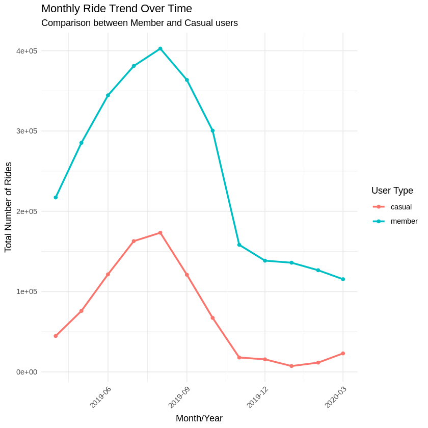
- A line chart clearly shows member stability vs. casual spikes.
- A histogram of trip durations shows the stark difference in ride intent (14 vs. 60 minutes!).
- A side-by-side bar chart makes it easy to spot which days need more bike redistribution.
Key Tasks Completed:
- Created visual breakdowns of user types by day and duration.
- Identified the audience: marketing stakeholders and product managers.
- Structured a clear narrative showing contrasting behaviors.
- Calculated usage proportions, daily averages, and variation percentages.
- Created charts to visualize weekday/weekend usage and trip durations.
- Identified top start/end stations and their significance for both user types.
- Analyzed peak ride hours for both member and casual riders.
Deliverable: Visualizations and Key Findings
I’ll export my visuals (e.g., plots of weekday vs. weekend usage by user type, average trip duration by user type, heatmaps of popular stations) and summarize the main conclusions alongside them.
🧭 Final Insight:
“Two riders pedal through the same city — one chasing the clock, the other chasing the moment.” To thrive, Cyclistic must embrace both. We now understand when, how, and why each type rides — and that empowers us to design smarter services, targeted campaigns, and better experiences.
# Let's visualize the number of rides by rider type
df_all_2 %>%
  mutate(weekday = wday(started_at, label = TRUE)) %>%
  group_by(member_casual, weekday) %>%
  summarise(number_of_rides = n()
            ,average_duration = mean(ride_length)) %>%
  arrange(member_casual, weekday)  %>%
  ggplot(aes(x = weekday, y = number_of_rides, fill = member_casual)) +
  geom_col(position = "dodge")
[1m[22m`summarise()` has grouped output by 'member_casual'. You can override using the
`.groups` argument.
# Count rides per hour and user type
hourly_usage <- df_all_2 %>%
  group_by(member_casual, start_hour) %>%
  summarise(ride_count = n(), .groups = 'drop')

# Find the peak hour(s) for each user type
peak_hours <- hourly_usage %>%
  group_by(member_casual) %>%
  slice_max(order_by = ride_count, n = 1) # Gets the hour with the most rides

# Visualize the hourly distribution
ggplot(hourly_usage, aes(x = start_hour, y = ride_count, fill = member_casual)) +
  geom_col(position = "dodge") + # Bars side-by-side
  # Or use facet_wrap for separate plots:
  # geom_col() +
  # facet_wrap(~member_casual, ncol = 1, scales = "free_y") +
  labs(
    title = "Distribution of Rides by Hour of Day",
    subtitle = "Comparison between Member and Casual users",
    x = "Hour of Day (Ride Start)",
    y = "Number of Rides",
    fill = "User Type"
  ) +
  scale_x_continuous(breaks = seq(0, 23, by = 1)) + # Ticks for every hour
  theme_minimal() +
  theme(axis.text.x = element_text(angle = 45, hjust = 1))

# --- Analysis 2: Seasonality and Monthly Trends ---

# Extract Month and Year (or create a Month/Year column)
df_all_2 <- df_all_2 %>%
  mutate(
    start_month = month(started_at, label = TRUE, abbr = FALSE), # Month name
    start_year = year(started_at),
    year_month = floor_date(started_at, "month") # Date truncated to the start of the month
   )

# Count rides per Month/Year and user type
monthly_usage <- df_all_2 %>%
  group_by(member_casual, year_month) %>%
  summarise(ride_count = n(), .groups = 'drop') %>%
  arrange(member_casual, year_month) # Sort for line plots

# Count rides per Month (aggregating all years - for pure seasonality)
seasonal_usage <- df_all_2 %>%
  group_by(member_casual, start_month) %>%
  summarise(average_daily_rides_month = n() / length(unique(start_year)), # Avg daily rides per month
            total_rides_month = n(),
           .groups = 'drop')


# Visualize Monthly Trends Over Time
ggplot(monthly_usage, aes(x = year_month, y = ride_count, color = member_casual, group = member_casual)) +
  geom_line(linewidth = 1) +
  geom_point() +
  labs(
    title = "Monthly Ride Trend Over Time",
    subtitle = "Comparison between Member and Casual users",
    x = "Month/Year",
    y = "Total Number of Rides",
    color = "User Type"
  ) +
  # --- CORRECTED LINE ---
  # Use scale_x_datetime because year_month is POSIXct (datetime), not Date
  scale_x_datetime(date_breaks = "3 months", date_labels = "%Y-%m") +
  # --- END CORRECTION ---
  theme_minimal() +
  theme(axis.text.x = element_text(angle = 45, hjust = 1))

# Visualize Seasonality (Average Annual Pattern)
ggplot(seasonal_usage, aes(x = start_month, y = total_rides_month, color = member_casual, group = member_casual)) +
  geom_line(linewidth = 1) +
  geom_point() +
  labs(
    title = "Average Ride Seasonality",
    subtitle = "Total rides per month (aggregated across all years)",
    x = "Month",
    y = "Total Number of Rides in Month",
    color = "User Type"
  ) +
  theme_minimal() +
  theme(axis.text.x = element_text(angle = 45, hjust = 1))

# --- Analysis 3: Most Popular Start/End Stations ---

# Define how many top stations to show
top_n_stations <- 10

# Most popular START stations
top_start_stations <- df_all_2 %>%
  group_by(member_casual, from_station_name) %>%
  summarise(start_count = n(), .groups = 'drop') %>%
  group_by(member_casual) %>% # Group again to get top N for each type
  slice_max(order_by = start_count, n = top_n_stations) %>%
  arrange(member_casual, desc(start_count))

# Most popular END stations
top_end_stations <- df_all_2 %>%
  group_by(member_casual, to_station_name) %>%
  summarise(end_count = n(), .groups = 'drop') %>%
  group_by(member_casual) %>%
  slice_max(order_by = end_count, n = top_n_stations) %>%
  arrange(member_casual, desc(end_count))

# (Optional) Most popular START-END station pairs
top_station_pairs <- df_all_2 %>%
  group_by(member_casual, from_station_name, to_station_name) %>%
  summarise(pair_count = n(), .groups = 'drop') %>%
  # Filter out trips starting and ending at the same station (optional)
  # filter(from_station_name != to_station_name) %>%
  group_by(member_casual) %>%
  slice_max(order_by = pair_count, n = top_n_stations) %>%
  arrange(member_casual, desc(pair_count))

# Visualisation of Top Stations (Example for Start Stations)
 ggplot(top_start_stations, aes(x = reorder(from_station_name, start_count), y = start_count, fill = member_casual)) +
   geom_col() +
   facet_wrap(~member_casual, scales = "free_y", ncol = 1) + # Separate plots
   coord_flip() + # Flip axes for better readability of names
   labs(
     title = paste("Top", top_n_stations, "Start Stations by User Type"),
     x = "Start Station",
     y = "Number of Rides Started",
     fill = "User Type"
  ) +
  theme_minimal() +
  theme(legend.position = "none")

🎯 ACT PHASE
🚲 Cyclistic: A Dual-Track System – Insights & Strategic Recommendations
Guiding Conclusion: Cyclistic serves two user ecosystems with almost opposite patterns:
Our analysis reveals Cyclistic serves two distinct user groups with almost opposite patterns:
-
🔹 Members:
- 81.3% of trips happen on weekdays.
- They ride an average of ~483,586 times per weekday.
- Trip durations are short: ~14 mins (weekday), ~16 mins (weekend).
- Use is consistent and utilitarian—primarily commute-focused.
-
🔸 Casual Users:
- Weekend rides account for 43.3% of their total trips (vs. 18.7% for members).
- Weekend average: 195,417 rides/day—a +91.1% surge compared to weekdays.
- Trip durations hover around ~60 minutes, regardless of the day.
- Use is leisure-driven: long rides, spontaneous, weather-dependent.
Conclusion: We don’t have “a user”—we have two. They need different pricing, different messaging, different bike placement—and a different vision.
Applying Our Insights: Strategic Actions
Here’s what the numbers are screaming:
🛠 Product & Pricing Enhancements
- Flexible Memberships: Offer seasonal or monthly memberships like “Your Summer Riding Pass” to attract casuals who avoid year-round commitments. Consider trial offers, e.g., “First month for £1.”
- Value for Leisure Riders: Promote longer ride durations in premium tiers or include 45-60 minutes in base plans, as casual users’ trips often hover around ~60 minutes. Promote ride-time tiers based on user history (e.g., frequent long rides).
📈 Data-Informed Campaigns & Targeted Messaging
- In-App Ride Data & Prompts: Use in-app ride data to target users in real-time. For instance, when someone rides 60 minutes on a Saturday, pop up with a message: “You spent £6 today—this same ride costs £0 as a member. Wanna ride smarter?”
- Segmented Targeting: Segment and target users who’ve taken 3+ weekend rides in a month—they’re ripe for conversion.
- Reframing Membership for Leisure: Develop messaging that reframes membership from “just for commuters” to “your all-access leisure pass.” Run ads with slogans like: “Ride More, Explore More, Spend Less” or “Membership: Because Saturdays Deserve Speed Too”.
- 🚲 Rider Behavior & Loyalty Campaigns:
- Looping Behavior: Many rides start and end at the same station (e.g., Streeter Dr & Grand Ave to itself, 7,470 rides). These are likely tourists or fitness riders doing circuits—perfect for promoting guided route suggestions or group discounts.
- Frequent Pair Riders: Track repeat pairings like “Lake Shore Dr & Monroe St → Streeter Dr & Grand Ave” (9,060 times) as an indicator of loyalty.
- “City Circles” Campaign: Launch a campaign called “City Circles” to reward loops and top start-end pairs with gamified badges, discounts, or tier progression.
🔧 Dynamic Bike Redistribution
- 📍 Station Hotspot Customization: Let data steer the fleet.
- Weekdays: Focus inventory near high-frequency commuter stations (Clinton, Adams, Madison) and workplaces, where ~483,586 member rides/day occur.
- Weekends: Shift bikes to parks, lakefronts, and tourist hotspots (Streeter, Monroe, Millennium Park), where casual riders generate ~195,417 trips/day (+91.1% surge compared to weekdays). Don’t leave bikes in the wrong places.
🥇 My Top Three Recommendations for Stakeholders:
- Flexible Memberships: Casuals ride ~195k times/day on weekends. Monthly/seasonal offers tap into this segment’s potential without long-term pressure.
- Targeted Messaging for Leisure Users: Trip duration for casuals is ~60 min—4x longer than members. They seek joyrides, not just commutes. Speak their language and promote campaigns like “City Circles”.
- Dynamic Bike Redistribution: Weekday: ~483k member rides/day. Weekend: ~278k casual rides/day. Don’t leave bikes in the wrong places. Let the data steer the fleet.
🧳 My Final Words for Stakeholders
This is more than data. It’s a compass. Cyclistic isn’t a one-size-fits-all service. It’s a dual-track system—and our strategies must reflect that. With smart segmentation, seasonal offers, and targeted rebalancing, we don’t just grow—we evolve.
Let’s turn insight into impact. 💼💥